Neural Computing pt 2: Sparse Distributed Representations
Hierarchical Temporal Memory (HTM) is a theory of the brain that I find fascinating.
Other attempts to model or explain the brain often lack detail, or attempt to force square pegs like well-understood mechanisms (backpropagation, etc.) into the round holes of biology, making ridiculous claims about undiscovered and completely implausible mechanisms while discarding the other 99% of observed mechanisms in the brain as irrelevant details or obvious biological mistakes.
While HTM certainly has its gaps, it is also directly confronts the complexity of the brain and attempts to discard little (at least when it comes to the cortex). It also has a peculiar property I rarely see; it feels organic. It doesn’t feel at all like the kind of thing a human would have ever designed; it breaks too many of our many implicit design rules, and it combines mechanisms in ways that are highly counter-intuitive while also paying off tremendously.
There used to be a common notion in AI research, one that bled into science fiction and popular culture, that the human brain is a sloppy, imprecise, unimpressive machine, and that precise, rigorous, logical computer AIs would rapidly overtake humans in all abilities. This is the trope that created many Twilight Zone plots and classic AI characters like HAL 9000.
To some extent, that notion is still around in some form. We do seem a little more willing to accept that biology has important lessons - after all, the state of the art of modern AI is based on “neural networks”, even if they have only a very vague resemblance to actual biology.
I strongly suspect however that the space of computational tools is vastly larger and more fascinating than we realize, that humans in the past century have only stumbled upon the tip of the iceberg, and that many of the greatest lessons about computation that we have yet to learn will be found in studying computers that were not designed by us, like the brain.
Making Sparse Distributed Memory Even More Sparse
If you haven’t read it yet, I’d suggest reading the original Neural Computing article on Sparse Distributed Memory. As we continue on in this article, we will be largely building upon the foundation of ideas and intuitions described there.
The sparse in Sparse Distributed Memory refers to the fact that the neurons can be viewed as addresses in a large address space, and that the addresses which produce a perfect match for one of these neurons are very few and far between.
However, if we consider the output vector of an SDM unit, where each bit encodes whether or not its corresponding neuron fires in response to the current input, we also notice that often this bit vector is sparse in a different way; that being that only a small percentage of neurons are likely to respond to any arbitrary stimulus, and so this output vector is almost entirely zero bits.
At first glance, this may appear to introduce inefficiency. The entropy of our encodings are very low relative to if we had denser representations. This may be true, but the same can be said about many problems subject to the space-time tradeoff. In this case, SDRs are trading space efficiency for a variety of wonderful properties.
At the foundation of HTM theory is the Sparse Distributed Representation (SDR), which refers specifically to the large bit vectors that HTM encodes data with. The sparse in SDR specifically refers to this second notion of sparsity, though both notions of sparsity here apply.
Similarity Function
This however is not the only difference between the SDRs of HTM theory and SDM. Another factor that changes is the distance function, which in HTM theory is more of a similarity function. Rather than take the Hamming Distance, we instead measure the number of overlapping bits between the two SDRs we are comparing.
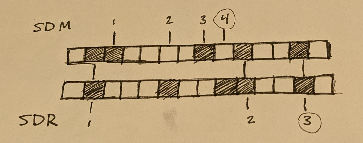
sdm_distance(a, b) = popcount(xor(a, b));

sdr_distance(a, b) = popcount(and(a, b));
Those among you with a keen eye and a linear algebra background may notice that, when applied to binary vectors, this is equivalent to a dot product. Let this guide your intuition ahead if you are so inclined.
Another perspective we can take here though is that this looks vaguely similar to the matching function used in a Bloom Filter. However, rather than the usual approach taken with bloom filters of looking for exact matches, with SDRs we count the precise number of matching bits, allowing us to differentiate between different degrees of partial matches.
When dealing with bloom filters, we normally are looking for perfect matches to maximize our confidence in having a correct match. However, the real world is noisy, and so we almost never will get perfect matches. So how much noise can SDRs tolerate?
(If you need a refresher on Bloom filters, this old article of mine gives a nice geometric intuition of how they work.)
Extraordinary Error Tolerance
Before going further, let’s look at some typical numbers from the brain.
Most cortical neurons have several thousand synapses. We can say roughly between 1000 and 4000 if we want good round numbers. This is the size of the SDR that each neuron is comparing the input SDR against. In practice, the input SDR may be much larger than this, and each individual neuron just looks at a subset of it.
Brain activity is remarkably sparse (granted, there are notable exceptions). In most cases, only a very low percentage - perhaps 1 or 2 percent - of neurons will be firing in a given brain region at any point in time. This of course does vary though, and can be somewhat higher as we will discuss later.
Given an SDR, this gives us two rough parameters we can use, commonly described as n and w. The size of the SDR, n, is simply the number of neurons/synapses involved, which is usually around several thousand. The number of nonzero bits, w, is usually on the order of 20-40, though we’ll talk about some flexibility here a little later. We can also derive a third parameter, s, which denotes the sparsity and is defined as w/n of course.
I’ll gloss over the precise mathematics of SDRs here as they get very complex very quickly, especially when dealing with partial overlap. Instead, I’d like to focus primarily on providing intuition with some rough approximations.
If we have an SDR where n=1000, w=20, and s=2%, the odds of picking any individual bit at random and getting a match is 2%. Picking multiple random bits and getting matches on more than one bit is exponentially less likely, as we have a roughly 2% chance of getting a right pick every time.
This is analogous to a bloom filter that has had very few elements inserted, so its false positive rate is extremely low.
If we require a 50% match on an SDR - which is an enormous amount of error tolerance mind you; half of our input bits can be replaced by random noise - the odds of getting a false positive here (correctly matching on 10 out of our 20 nonzero bits) are only about 10^-13, or about 1 in 10 trillion.
If our noise is only 30% and we decide we can demand 14 bits to match rather than 10, this drops to 10^-23. A perfect match on all 20 bits is about 10^-42.
Compare this to a dense representation like standard SDM, where zero and nonzero input bits are often split roughly 50/50. This may offer more efficient computing in some sense, but the difference between the bitvector for any given neuron and a random input is statistically close to 50%. Add in a little sparsity, and that quickly gets close to 0%.
Superposition and the Union Property
In many cases, this amount of error tolerance is a bit excessive. In the event that a neuron does fire in error, the effect is that a single bit of noise is added to the output SDR for this group of neurons. The next cortical region in the larger brain circuit that receives this input can certainly tolerate a single bit of error. We’ve established already that it can tolerate a lot more than that.
So can we trade some of this error tolerance for something else? Of course!
Seeing as SDRs behave in many ways like bloom filters, we can exploit another property of bloom filters, albeit one that gets relatively little attention; the union operation. We can take multiple bloom filters of equal sizes and identical hashing functions and apply a bitwise OR operation to unify them into a single, denser filter. This is equivalent to creating a new bloom filter that contains all of the values inserted into both input filters. It retains its properties of guaranteeing only false positives, though the substantial increase in density has probably increased our false positive rate by a fair margin.
Before discussing what it means to combine SDRs like this, let’s note exactly what an individual SDR is actually encoding.
A large amount of intelligence is categorization. If you’re not categorizing what something is, you’re probably categorizing where it is or how you should interact with it.
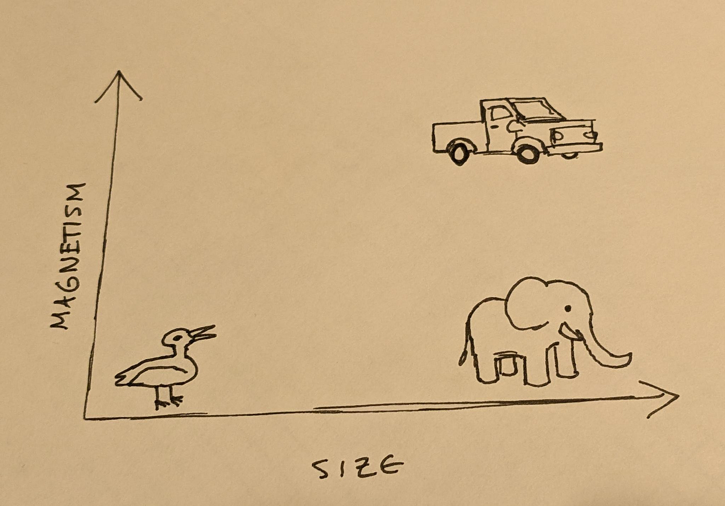
You might be able to tell a duck and a truck apart by size alone, but separating trucks and elephants by just size may give you some trouble. If you take into account another factor, say, magnetism, we can then separate these categories.
Of course, all of these things vary in size; baby animals are smaller than adults, and modern trucks are often a lot bigger than older trucks. Each of these categories is not a point, but a cluster or manifold of points. Accurately separating categories requires drawing lines between clusters in very high numbers of dimensions. Many of these dimensions may be as mundane as something like “color of pixel at some specific X,Y coords”. Many other dimensions may be derived from data across other dimensions; for example, if we added more animals of varying sizes to the above plot, we could probably group them all into a big “animals” cluster. A set of neurons that recognize when something is in that cluster could be used as an “animal” dimension that could inform more complex judgements.
The clusters are also not guaranteed to be spherical, nor always cleanly separated. In fact, pretty much any way you can imagine making them weirdly shaped, twisted, coiled, entangled with each other, etc. tends to happen with some set of categories on at least some occasion.
One notable difference between brain-inspired models and modern deep learning models is that DL tends to categorize things by drawing lines between them and having its “neurons” output a number between 0 and 1 based on which side of the line the input is on. Brain-based models tend to stick a neuron in the middle of the cluster and have that neuron fire whenever the input is sufficiently close.
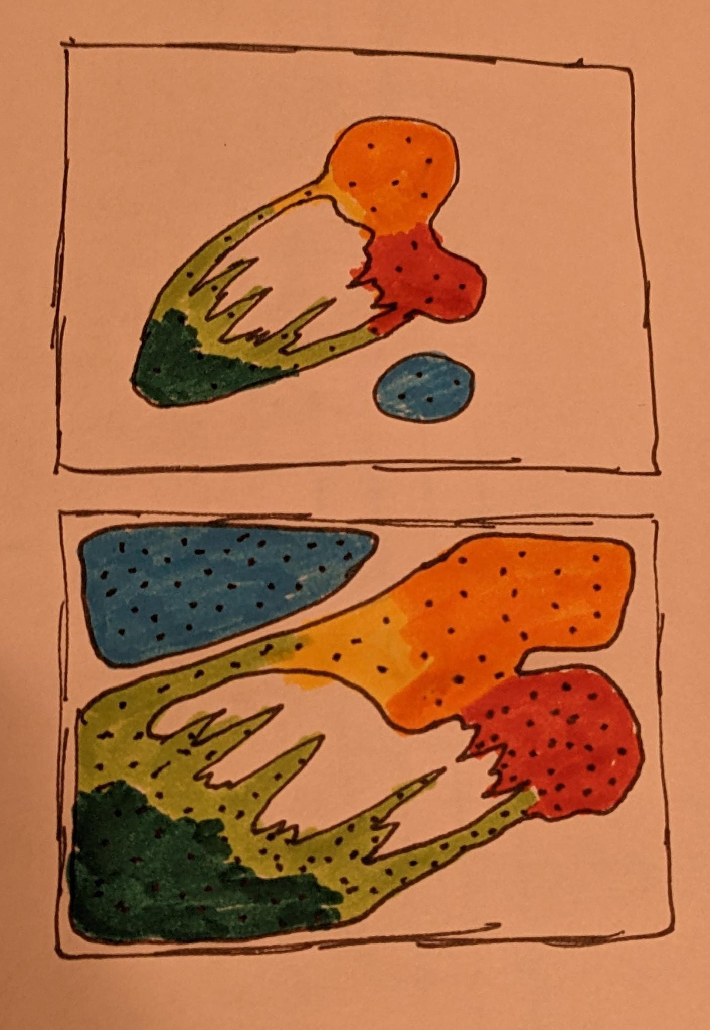
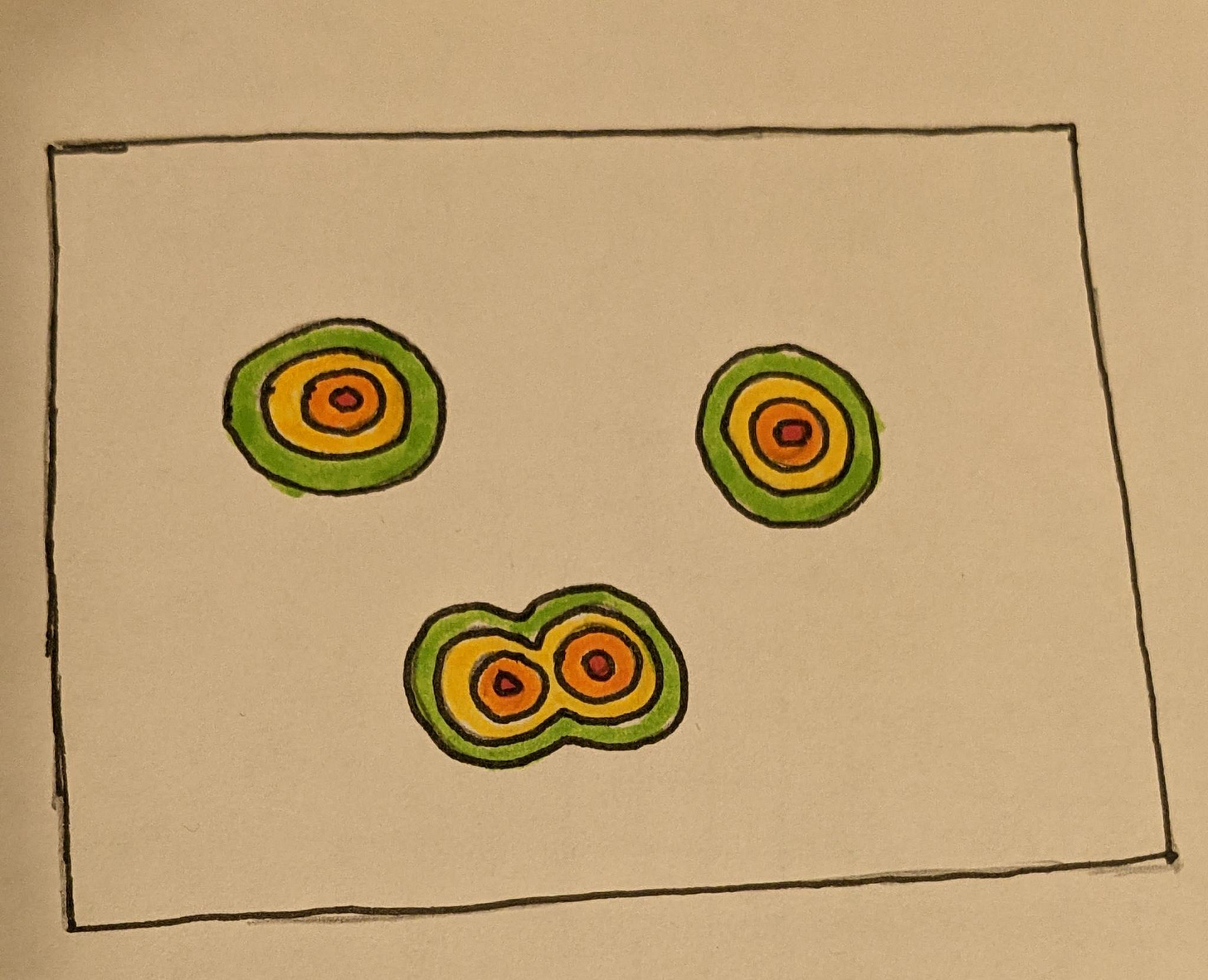
We can think of this categorization problem that the brain is doing as creating a very large, very high-dimensional scatter plot of all of our input values, and placing landmarks near different clusters and interesting points. An encoding in SDM or an SDR is then just some list of nearby landmarks to this point, some of which might be recognized to us as being analogous to features or categories, even if we might not have words associated with every one. If there is a particular region of this scatter plot that we want a higher-resolution map of, we can pass this location encoding to another brain region, which can then map it out in even more detail.
What an SDR represents is an encoding of the current input being perceived, and how it relates to known, familiar concepts. In some sense, this is an approximate location on one of these manifolds or clusters.
If we then take the union of several SDRs, we are representing multiple locations in this space at once, effectively multiple objects we can model at the same time.
Of course, doing so reduces the sparsity of our SDRs, which negatively impacts our error tolerance. Specifically what is going on is that we are representing multiple possibility bubbles around each object to account for noise, and these bubbles can begin to bleed into each other when these objects are similar (close) enough.
I’m sure everyone has plenty of experience with how much easier it is to make mistakes and misjudgements when their working memory is pushed to its limits.
One way in which HTM exploits this that we will talk about next time is in representing ambiguity. We can represent forking paths of possibilities that we can’t yet rule out, and then begin pruning them away as new information starts conflicting with some. If you see something moving around in the bushes, your visual cortex may come up with a complex superposition of possible scenarios of what it might be, and then when a meow is recognized by the auditory cortex and that signal ripples throughout the brain, that superposition collapses to a single feline possibility.
Takeaways
There are some other properties of SDRs that I intended to discuss here, though this article is already pretty long (and a day overdue). In particular I wanted to discuss some interesting properties of modelling manifolds with the unusual geometries that sparsity creates, though I think that might be best saved for a future article on grid cells perhaps. There are a few other articles on HTM in this series that I’ll have to write about first though, as we’ve only scratched the surface of its complexity.
In particular, we’ve described probably about 90% of the “spatial pooler” in HTM here. For the next installment in this series I intend to talk about HTM’s spatial pooler and temporal memory.
With that said, SDRs are a rather unusual combination of mechanisms that I have a hard time imagining human would have created any time soon without some kind of external inspiration like the brain.
Yes, bloom filters offer a nice and somewhat familiar framework for understanding them, but we’re largely using them in unfamiliar ways. We’re not looking for exact matches, but partial matches which are much more complex to model mathematically. We’re not slowly saturating the filter over time, but rather we’re representing a value or combination of values at a specific time before replacing it with a new representation of the next incoming data. We’re then exploiting the rather obscure union property of bloom filters for multicomputation, superpositions, and as we’ll see next time ambiguity and its resolution.
All of these properties meld together into a rather complex but extremely flexible computational tool, one where all of these properties to some extent rely on or produce each other. There also are very fuzzy extreme cases; a human would likely have tried to generalize this into something with a union property that doesn’t just lose all precision when pushed to extremes (the brain has its own mechanisms for preventing this, though they might not meet human demands for elegance).
I also suspect that it’s not easy to engineer SDR-based systems, at least with existing tools. Numenta, the research company behind HTM, has developed “encoders” to map human-familiar data into SDRs, though they struggle with doing the inverse. I suspect that various forms of synthesis-based programming will need to fill this gap before manual engineering becomes practical.
Regardless, this is a very fascinating computational tool, one that I hope to portray as even more fascinating over the next few Neural Computing articles, and one that I hope provided you a glimpse of the weird possibilities beyond the familiar human-style computing around arithmetic on binary-coded integers.
Those might take a little while though, as I think I might need to write a fair bit of code to do it justice.
Thank you for reading this article, it took a fair bit more work than I expected, which is why it’s a day late. I’m going to try to get another neuro-themed article out soon (hopefully later this week) giving my thoughts on Neuralink’s newest show-and-tell, as well as some thoughts on the company in general.
If you enjoyed this article, subscriptions (both free and paid) are greatly appreciated. I’ve been playing a bit with the chat feature on the substack app, so definitely check that out as well for updates, discussions, feedback, and questions.

