Programming in Hyperspace pt 2
[A repost from my old Medium blog]
This article is a repost of an article I wrote on Medium in 2019. Part 1 was reposted earlier this week. I wouldn’t consider this my best work, this part especially gives some useful background and geometric intuition that should prove very useful for the next couple entries in my Neural Computing Article. The beginning of part 1 also hints slightly at some of the unique ways in which I’ve been trying to rigorously think about software development and how to improve the process.
There are also some loose threads and unresolved problems I mention across these two articles that I have found some more satisfying answers to in the past 3 years, which I’ll probably write about here eventually. I have quite the backlog.
Enjoy!
Okay, in part 1 I went over some strange applications of bitwise operations; mostly some unique number theory stuff for dealing with repetitive bit patterns, doing horizontal adds, and doing some strange, more obscure operations.
This time, we’re going even deeper down this rabbit hole, but this time with a special focus on some properties of Bloom Filter -like data structures. Some of the stuff in this article is even used in production, so you’ll probably find some more practically useful things here compared to last time.
Review of Bloom Filters
Let’s just quick review bloom filters here, as a lot of the rest of this article is built upon strange variations of them.
A bloom filter is a type of probabilistic data structure. It acts like a set with a lookup operation that guarantees no false negatives, but sometimes provides false positives.
In other words, it has a lookup operation that answers either “definitely no” or “maybe yes”.
Bloom filters are also quite fast, and have a fixed storage size; a bloom filter containing one item might take up just as much space as one containing a million. This of course comes with a trade-off; the more data you try to pack into a small amount of space, the less precise it gets and the higher the probability of a false positive. There is a trade-off between accuracy and size, and the exact parameters you need can be easily tuned.
They can be useful as a cheap and fast approximation of a more expensive search. For example, Google at one point used them in Chrome to detect if a website was malicious; searching any URL in a database of malicious sites was too expensive to do for every website, so they instead used a bloom filter to quickly sift out most websites. If a URL was not found in the bloom filter, it meant it wasn’t in the database. If it was found in the bloom filter, that meant that it could be in the database, and so the expensive database check was done to make sure.
Bloom filters are nice for approximations of much more expensive operations. As we’ll see throughout this article, bit manipulation can be used to create quite a lot of interesting approximation techniques.
How do they work?
Take a bit vector of N bits. Set all bits to be zero. This is your empty bloom filter.
To insert an object, you first generate a hash of the object. Treating the hash as an integer, we can use it to select an index within the bit vector. Set the corresponding bit to 1. We have now inserted our object into the bit vector. If we want to check if an object is in the bloom filter, we simply hash it and check if the corresponding bit has been set.
Assuming we have a good hashing algorithm, we should have roughly a 1/N chance of getting a false positive.

As we insert more objects, the chances of a false positive increase. Due to some properties of random numbers, a bloom filter with N bits will have roughly a 36.78% chance of a false positive after N element have been inserted.
However, we can actually improve this. Suppose we had a second bloom filter that used a different hash. In this case, the problem changes from finding one matching bit to finding two. Say we have a bloom filter with a 20% chance of a false positive. If we increase this to 2 bloom filters that both have to pass (and importantly use different hashes), then that probability drops to 20% * 20%, or 4%. If we increase this to 3 filters with a 20% false positive rate, that drops to 0.8% total. As we increase the number of hashes to check, the likelihood that any particular object will pass multiple filters drops exponentially with each additional filter.

In practice, multiple separate filters aren’t used. Instead, we might have a Bloom Filter with N bits and K hashes, and set K bits for each inserted object. This means that the filter fills up K times faster (so make it K times bigger), but the odds of a false positive are actually a bit lower when what we have is essentially several large, overlapping filters rather than several small, independent filters.
At the Heart of the Bloom Filter
Let’s deconstruct the bloom filter a bit, and see if there are some unique properties we can steal.
Mutable Constraint Models
Constraint systems are like magic, even if they break a few rules.
Imagine you’re trying to design a rocket to go to Mars. How do you do that? You could spend a fortune, and direct thousands of engineers over several years to accomplish that goal. Or, if you had a smart enough constraint solver, you could give it some rules about physics, and a few constraints along the lines of “go from Earth to Mars within X months”, “limit G-forces to 3Gs” (to keep astronauts safe), and “cost < $1,000,000,000”. And if it’s smart enough, it might spit out a rocket design in a reasonable amount of time.
That design might not be airtight (you didn’t add a constraint about that, now did you?), so all your astronauts might quickly asphyxiate, but other than that, it still seems to be a viable rocket design.
Constraint systems, simply put, are a declarative way of building things. You define the problem by listing requirements, and you get a solution by finding something that satisfies all those requirements.
Software that solves these kinds of problems exist. Look into SAT (Boolean SATisfiability Problems) solvers and SMT (Satifiability Modulo Theories) solvers for examples. Of course, in practice, solving these kinds of constraints is hard. Like, really hard. Typically NP (exponential time) or worse. Often, there are quite a lot of shortcuts that can be taken, and ways of making things much easier when certain assumptions can be made, making problems generally a lot easier than they look, though it can still get really hard in the general case.
Luckily, we’re not interested in “solving” the constraint system. Rather, we’re interested in detecting when something satisfies our constraints. It’s much easier to test if a particular rocket can go to mars than it is to design one that does. The reason why constraint solving can get hard is because sometimes the only way to find a solution is to check every possibility until you find one that works.
Sum Constraints
The specific way that Bloom Filters handle constraints is interesting, and opens up a lot of room for flexibility.
Here, the constraints are done with the bit vectors. If we have N bits, and assuming our hashing function is good, each 1 bit allows 1/N of the space of possible values through the filter. Each 0 bit blocks 1/N of the spaces.
It’s like we have N constraints we can toggle on and off (though typically in a Bloom filter, we can’t really safely turn a 1 bit back into a 0).
We could perhaps build something a bit like a Bloom Filter that used non-hashing constraints. We could, for example, build up a large set of rules that values we insert pass, and update those rules whenever we insert a new item. That’s hard though, and can get complicated really fast. The elegance of this constraint format is its simplicity. The hashes map random subsets of our input space to individual bits, which we can toggle on and off.
Shadows
Another thing we can notice is the effect that multiple hashes have. Even if an incorrect value happens to pass through one set of constraints, the odds of it passing another are pretty low. They get lower with every additional constraint we add.

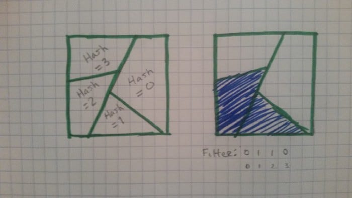
Another way to think of this is as such; the data we are storing in the bloom filter is a bit like a geometric object. However, rather than store the entire object, we instead store “shadows” of the object. Each new hash is a “shadow” from a different perspective. With enough perspectives, we can reconstruct a pretty detailed model of the object. The actual object isn’t the shadows, but rather some subset of the space where all of the shadows intersect.
There is some space where the shadows intersect, but where our object doesn’t lie. This is where our false positives come from. Of course, there are no places where our object lies, but where it doesn’t cast any shadows, so we don’t get any false negatives.
At this point, we’re not representing our problem by all the places it is, but rather we’re representing it with constraints, and by defining it in terms of known places where it isn’t.
As mentioned before, constraint systems can sometimes be really hard to solve. In this interpretation, “solving” is when we want to directly observe the object — translating between a collection of shadows, and the actual object they are cast by.
Shadows of Dustclouds
In practice, the shadows we generate from a bloom filter are actually rather unlike the shadows we see in real life. The objects we see in real life are rather continuous; they are made up of many points that are close together, with few gaps in between. This means that shadows are also quite continuous, and that a shadow isn’t just cast by a single point, but also by many of the points around it.
However, the space of possible objects we are working with are often quite big. Unfathomably big. Any object you insert into the bloom filter is just a single, extremely tiny point in that vast space.
Yet, it casts a shadow. If your bloom filter is N bits, and you use k hashes, each object takes up roughly (100 * k/N)% of that space. For a point that takes up such an infinitesimally minuscule space, that’s a big shadow. As a result, your bloom filter might start to fill up fast.
Another issue is that objects that are similar to each other will likely generate completely different hashes. So if you pack a lot of similar objects into the bloom filter, it fills up just as fast as if you insert random objects. Instead of nicely cutting up spaces like the diagrams in this article show, it’s like our hashing algorithms are tossing our space into a wood chipper.
So what if we change the hashing algorithm?
Structure-Sensitive Hashing and Grid Filters
Let’s say we want to use something similar to a bloom filter to approximate a problem where we’re working with continuous data. Say for example we want to check if a particular point is inside of some complex 3D object.
We can’t just iterate over all the points that lie within the object and insert them all into the bloom filter. There’s a massive number of individual points that will fall into there. Creating such a bloom filter would be extremely expensive, likely take exponential time, and would likely fill the bloom filter entirely, no matter how big we make it.
So let’s change the problem. Let’s use a hashing algorithm designed specifically to get us false positives, but mostly within specific circumstances that work in our favor.
Say we overlay a grid onto the object, and map every space in the grid onto a bit in our bloom filter. We can then use something similar to rasterization to fill in all the spaces in the grid that have at least some part that overlaps with our object. Such an algorithm would scale linearly with the number of spaces in our grid.
Of course, there will be some spaces on the grid where there is some overlap, but not much. So let’s rotate the object relative to the grid, then repeat the process to generate a second grid.
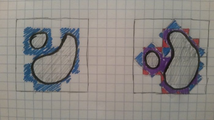
This is similar to casting a shadow from another angle in the example we gave before. This has the effect of rounding off some of the sharp, stair-stepped edges of our object, and can cut out many of the spaces where there’s overlap.
Of course, this also changes the problem from one about shadows of dustclouds to shadows of more continuous objects. This means that “similar” points actually tend to create overlapping representations, and we only actually fill up the filter if we come close to filling up the entire space of possible values. In other words, if our object takes up a lot of space.
But if that’s the case, does it matter? If our object fills up most of the space, then most points will not only pass the filter, but will also wind up in our object as well.
Some other properties this has are that 1.) more “shadows” or “hashes” actually gets diminishing returns, rather than improving accuracy exponentially, and 2.) for this particular example, the size of the grid has a big impact on how small of details it can represent, so scale your grid accordingly.
It’s also worth pointing out that this way of representing shapes is actually vaguely similar to the way that the Grid Cells in your brain are known to represent location (by using multiple overlapping grids at different relative scales and orientations), but that’s an explanation for another time.
As far as I’m aware, I’m the first person to invent this data structure (though I’m skeptical of this claim; if anyone knows of it being used somewhere else, let me know!). As its [presumed] inventor, I’ll name it a Grid Filter.
Sketches: Bloom Filters with Similarity Scores
This next data structure is one that I’ve seen with a couple different names, so I’m going to refer to it with the simplest one, a “Sketch”. If you’ve heard of Sparse Distributed Representations, or Sparse Distributed Memory, those are other names for this.
If you’ve been following Numenta for a few years, you might recognize this. The original idea for this predates their work with it by a couple decades, but it’s all really from the same source.
For those who haven’t heard of any of this, this is all stuff from the realm of theoretical and computational neuroscience. We’re literally talking here about the data structures that your brain uses.
Suppose we want to create a hash of a data structure. However, we want objects with similar properties to produce similar hashes so that we can easily calculate similarity scores between objects.
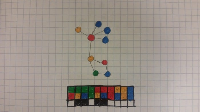
What we can do is create some kind of function that detects simple features or properties of a data structure that we find significant, and then maps them onto indices for a bit vector. We can then set all bits in the bit vector that relate to detected properties.
This can allow us to create compact summaries of data structures. It of course isn’t perfect. A large data structure packed into a small bit vector will lose a lot of information. Large data structures with a lot of variability will also likely fill most of the bits, making it hard to discern specific features. This approach also doesn’t store how many instances of a particular feature show up, just whether or not it does.
It’s also useful to consider what might be a “good” feature to track. For example, “The quick brown fox jumps over the lazy dog” includes every letter in the English alphabet, and thus would fill a bit vector that only looks at which individual letters appear.
If instead you look at subsequent pairs of letters, suddenly a lot of possibilities for rearranging a string disappear. In the aforementioned sentence, we have a lot of letters that only are ever followed by a single letter, meaning that we could reconstruct large portions of the string from just letter pairs. For example, if we see an l, we know it must be followed by a, then z, then y, and so on. We do eventually get to an o, which can be followed by w, x, v, or g, creating ambiguity.
At least when we’re dealing with relatively short strings, this preserves a surprising amount of structure in a relatively short bit vector.
We can then of course also bring into account the “shadow” properties again, and represent an object with multiple feature sets. This also adds more ways to measure similarity between objects.
Comparing Sketches
If you have two sketches that have a lot of bits in common, then that implies that they have a lot of features in common too. This kind of comparison can be done quite simply by performing an AND operation between the two sketches to get the bits they have in common, and then a POPCOUNT operation to get the number of set bits that are left.
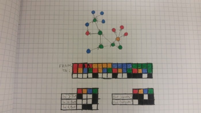
Another interesting property is that we can efficiently check for subsets. If we have sketches of two graphs, and we want to check if one is a subgraph of the other, we just need to check if its sketch is a subset. This is of course an approximation and will occasionally return false positives, but a couple of bitwise operations are far cheaper than actual subgraph checking algorithms.
Building on Top of This?
While I have yet to fully explore this space, I think there’s potential for more advanced data structures to be built on top of this. For example, if there were a way to perform a similarity score -based lookup, that may be useful for many applications.
I also think a tree-like data structure that allows for efficient lookup of subsketches would be useful. It appears as though such a data structure might be very useful for compiler optimization. This is something I’m looking into, but I don’t have anything concrete to show yet.
Locality-Sensitive Hashing: Object Classification without Machine Learning
Let’s say we want to do a similarity score-based lookup (k-NN style), and are willing to take a minor hit in accuracy (as in, we’re fine with occasionally missing a neighbor). Simply put; we have some set, and a sketch (or other input), and we want the top k elements of the set with the best similarity scores.
How can we do this efficiently? If we want perfect results, the problem unfortunately requires a linear search. However, when we can handle occasionally imperfect results, it turns out there’s a simple strategy based on hashing to do this; Locality-Sensitive Hashing.
If we have a dataset, we can imagine it filling some high-dimensional space. If our dataset consists of sketches, then each dimension actually represents a feature in our data.
The problem mostly becomes a matter of dividing up the space in a way such that points close together can be easily located in some kind of data structure. Interestingly, we can actually think of this a little bit like the Grid Filters we discussed earlier.
The Grid Filters work by looking at some object from a variety of random orientations and mapping each perspective to a grid. A point passes the filter if it matches with the object when viewed from every orientation. Let’s tweak that a bit.
Instead of mapping objects to grids at different angles, let’s instead divide the space in half with a random hyperplane. All points on one side of the hyperplane are one group, and all that lie on the other side are in the other group.
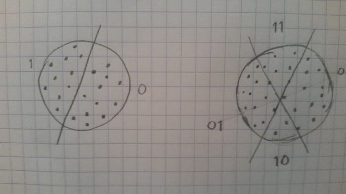
Using bit vectors, the simplest way to create a hyperplane is to just check the value of a single, random bit. All the sketches where that bit is a zero lie on one side of the hyperplane, and all the sketches where that bit is a one lie on the other side. There are other ways of dividing up the space, but this is probably the simplest.
We can divide things further with another random hyperplane. With two hyperplanes, we actually get 4 categories. If we throw N hyperplanes at the problem, we can build up an N-bit hash for a given point by setting each bit to a 1 or a 0 depending on which side of the corresponding hyperplane it lands on.
Because two points that are quite close together are likely to land on the same side of each hyperplane tested (the only way this wouldn’t happen is if the points just so happen to be quite close to one of them, which does happen occasionally), we can use this to create a locality-sensitive hash; a hashing algorithm with many of the familiar hashing properties, but that mostly ignores minor changes in the data.
We can then also use this hash to place objects into a hash table. This table will likely have a lot of collisions, so we likely will want to choose an implementation that handles collisions efficiently.
Now suppose we want to do a k-NN search. We hash our input sketch with this method, and then perform a lookup in our hash table. We then look through all the elements returned, and filter out all but the k elements with the highest similarity scores.
We might also want to search “nearby” hashes. What this means is we not only look up our hash in the hash table, but also all the hashes that differ by only 1 bit. If we have an N-bit hash, that’s N additional lookups to perform. This might sound expensive, but it mostly solves the aforementioned problem of nearby points occasionally winding up on different sides of single hyperplane. It also isn’t that bad; if we have a 16-bit hash, we’ll have to do a total of 17 lookups (the original hash + the 16 hashes that differ by a single bit), compared to searching through the whole 65536 hashes across the table. If we have a large dataset, this is way better than searching through every possible object.
If we scale to larger hashes, the improvement is exponential. If we had a 32 bit hash, we’d only need to look up 33 total hashes, out of over 4 billion.
There’s still some chance of missing some values. While unlikely, it could be that two nearby points happen to fall on different sides of two different hyperplanes. Remember though that this technique is approximate; it doesn’t guarantee perfect results. If we wish to get more accuracy, we could always check more hashes; for example, every one that differs by up to 2 bits. Or we could go up to 3. Or more. Of course, this gives us harshly diminishing returns, as the likelihood of a mistake drops exponentially and the number of hashes we need to check increases exponentially.
This technique is actually used in production quite often. Wikipedia gives a nice list of applications, but it’s generally quite good for “fingerprinting”, clustering, and classification problems that need to tolerate minor variability in data. In fact, most machine learning tasks amount to just fancy ways of solving these kinds of problems, so it’s quite interesting that we have a way to do it with no learning, and just hashing algorithms.
Future Work
I think there’s a lot of untapped room for experimentation here. These kinds of approaches are quite different from the common strategies that most programmers use, and show that there’s way more to Bloom Filters than people realize.
I think viewing these data structures as constraint systems is a useful perspective, and definitely needs more exploration. What kinds of other problems can we solve with similar techniques?
As we scale to larger and larger numbers of cores, we’re going to need to be able to keep all those cores fed with data. The problem is that computing power is much easier to scale than memory bandwidth, so the 1024-core CPUs of tomorrow will need to be careful with how they manage memory, or they’ll spend more time waiting on data than actually working. Packing more data into less space is a great way to do that, and so investigating new ways of representing data will soon become very valuable.
I expect that Grid Filters may be quite useful in a lot of simulation and gaming applications, as performance is critical there, and geometric operations can be quite expensive. I’m also wondering; could there be other ways of doing these structure-sensitive hashes to approximate other types of problems?
So I’ll end this article with a call to action: investigate these kinds of techniques more and look for similar kinds of tools! There’s a vast range of algorithms and data structures left to be discovered, and these kinds of systems seem to hint at a new frontier.
Next week’s article should be Neural Computing pt 2 : Sparse Bit Vectors, which is a more fleshed-out discussion of the “sketch” data structure described in this article, particularly how it can be applied to understanding how the brain computes.
If you’re new here and want to follow my work, you can follow below. Sharing my work and getting a paid subscription are also greatly appreciated!


